Datei:InterpolationBsp1.png
Aus DGL Wiki
Version vom 5. November 2005, 01:53 Uhr von Lyr (Diskussion | Beiträge) (Beispiel für Lineare Interpolation. Mathematica Code für diese Grafik: E1 = t*2 + 2 E2 = -4*t + 5 S1 = ParametricPlot[{E1, E2}, {t, 0, 1}, Frame -> True, GridLines -> Automatic, PlotStyle -> Thickness[0.01]] S2 = ListPlot[{{2, 5}, {4, 1}},)
Es ist keine höhere Auflösung vorhanden.
InterpolationBsp1.png (250 × 154 Pixel, Dateigröße: 1 KB, MIME-Typ: image/png)
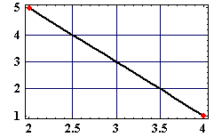
Beispiel für Lineare Interpolation. Mathematica Code für diese Grafik:
E1 = t*2 + 2
E2 = -4*t + 5
S1 = ParametricPlot[{E1, E2}, {t, 0, 1},
     Frame -> True, GridLines -> Automatic, PlotStyle -> Thickness[0.01]]
S2 = ListPlot[{{2, 5}, {4, 1}}, PlotStyle -> {RGBColor[1, 0, 0],
     PointSize[0.03]}]
Show[S1, S2, TextStyle -> {FontFamily -> "Times",
    FontSize -> 14, FontWeight -> Heavy}]
Dateiversionen
Klicke auf einen Zeitpunkt, um diese Version zu laden.
| Version vom | Vorschaubild | Maße | Benutzer | Kommentar | |
|---|---|---|---|---|---|
| aktuell | 01:53, 5. Nov. 2005 | | 250 × 154 (1 KB) | Lyr (Diskussion | Beiträge) | Beispiel für Lineare Interpolation. Mathematica Code für diese Grafik: E1 = t*2 + 2 E2 = -4*t + 5 S1 = ParametricPlot[{E1, E2}, {t, 0, 1}, Frame -> True, GridLines -> Automatic, PlotStyle -> Thickness[0.01]] S2 = ListPlot[{{2, 5}, {4, 1}}, |
- Du kannst diese Datei nicht überschreiben.
Dateiverwendung
Diese Datei wird auf keiner Seite verwendet.