Datei:InterpolationCosAnnaeherung.png: Unterschied zwischen den Versionen
Aus DGL Wiki
Lyr (Diskussion | Beiträge) (Cosinus-Interplation Annäherungen. Mathematica Code für diese Grafik: E1 = 1 - t^2*2 E2 = (1 - t)^2*2 S1 = Plot[ E1, {t, 0, 0.5}, Frame -> True, GridLines -> Automatic, PlotStyle -> RGBColor[0, 0, 1]] S2 = Plot[ E2, {t, 0.5, 1}, Frame -> True, ) |
(kein Unterschied)
|
Aktuelle Version vom 5. November 2005, 05:40 Uhr
Cosinus-Interplation Annäherungen. Mathematica Code für diese Grafik:
E1 = 1 - t^2*2
E2 = (1 - t)^2*2
S1 = Plot[ E1, {t, 0, 0.5}, Frame -> True, GridLines ->
    Automatic, PlotStyle -> RGBColor[0, 0, 1]]
S2 = Plot[ E2, {t, 0.5, 1}, Frame -> True, GridLines ->
    Automatic, PlotStyle -> RGBColor[0, 0, 1]]
S3 = Plot[(1 + Cos[t*Pi])/2, {t, 0, 1}, Frame -> True,
    GridLines -> Automatic, PlotStyle -> RGBColor[0, 1, 0]]
S4 = Plot[ 2*t^3 - 3*t^2 + 1, {t, 0, 1}, Frame -> True, GridLines -> Automatic,
    PlotStyle -> RGBColor[1, 0, 0]]
Show[S1, S2, S3, S4, TextStyle -> {FontFamily -> "Times", FontSize -> 14,
    FontWeight -> Heavy}]
Dateiversionen
Klicke auf einen Zeitpunkt, um diese Version zu laden.
| Version vom | Vorschaubild | Maße | Benutzer | Kommentar | |
|---|---|---|---|---|---|
| aktuell | 05:40, 5. Nov. 2005 | 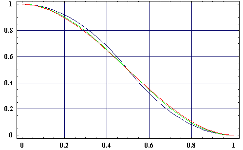 | 499 × 308 (2 KB) | Lyr (Diskussion | Beiträge) | Cosinus-Interplation Annäherungen. Mathematica Code für diese Grafik: E1 = 1 - t^2*2 E2 = (1 - t)^2*2 S1 = Plot[ E1, {t, 0, 0.5}, Frame -> True, GridLines -> Automatic, PlotStyle -> RGBColor[0, 0, 1]] S2 = Plot[ E2, {t, 0.5, 1}, Frame -> True, |
- Du kannst diese Datei nicht überschreiben.
Dateiverwendung
Diese Datei wird auf keiner Seite verwendet.